Neural Networks: All You Need to Know

The backbone of any large scale ML project starts with a Network… A Neural Network and Here’s all you need to know about them.

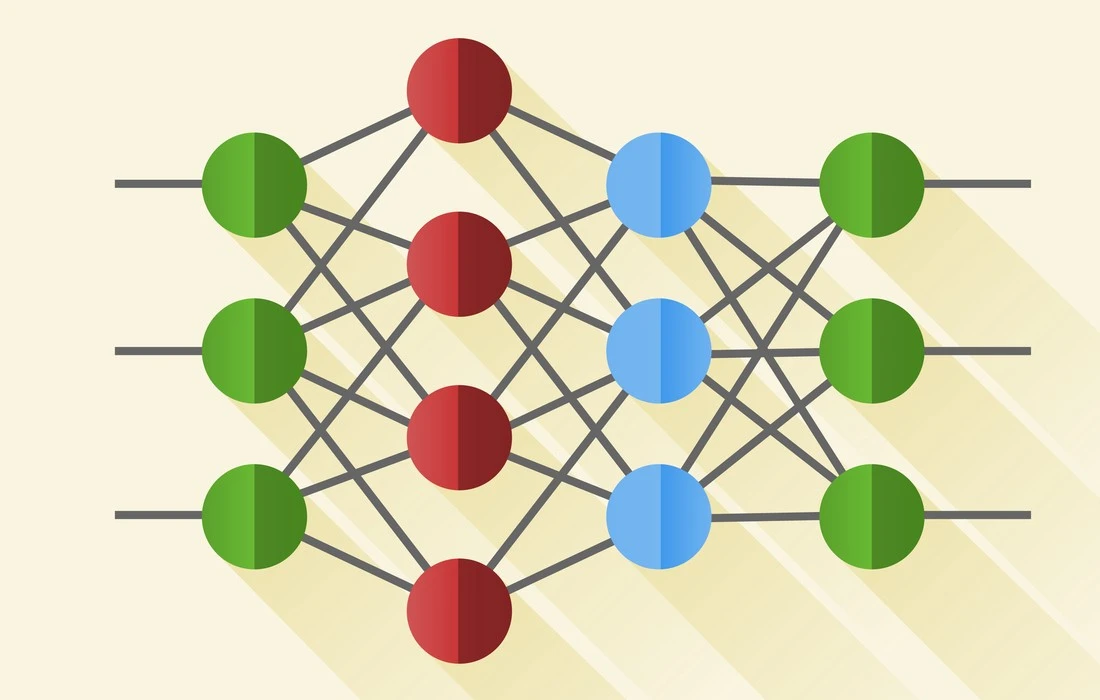
A Neural Network performing a prediction

As stated in the sub-title, Neural Nets(NNs) are being used almost everywhere, where there is need of a heuristic to solve a problem. This article will teach you all you need to know about a NN. After reading this article, you should have a general knowledge of NNs, how they work, and how to make one yourself.

Here’s what I will be going over:

History of Neural Nets
What really IS a Neural Network?
Units / Neurons
Weights / Parameters / Connections
Biases
Hyper-Parameters
Activation Functions
Layers
What happens when a Neural Network learns?
Implementation Details (How everything is manged in a project)
More on Neural Networks (Links to more resources)

History of Neural Nets

Since, I do not want to bore you with a lot of history about NNs, I will only be going over their history, very briefly. Here’s a Wiki article on the topic if you want more in-depth knowledge on their history. This section is majorly based off of the wiki article.

It all started when Warren McCulloch and Walter Pitts created the first model of an NN in 1943. Their model was purely based on mathematics and algorithms and couldn’t be tested due to the lack of computational resources.

Later on, in 1958, Frank Rosenblatt created the first ever model that could do pattern recognition. This would change it all. The Perceptron. However, he only gave the notation and the model. The actual model still could not be tested. There were relatively minor researches done before this.

The first NNs that could be tested and had many layers were published by Alexey Ivakhnenko and Lapa in 1965.

After these, the research on NNs stagnated due to high feasibility of Machine Learning models. This was done by Marvin Minsky and Seymour Papert in 1969.

This stagnation however, was relatively short-termed as 6 years later in 1975 Paul Werbos came up with Back-propagation, which solved the XOR problem and in general made NN learning more efficient.

Max-pooling was later introduced in 1992 which helped with 3D object recognition as it helped with least shift invariance and tolerance to deformation.

Between 2009 and 2012, Recurrent NNs and Deep Feed Forward NNs created by Jürgen Schmidhuber’s research group went on to win 8 international competitions in pattern recognition and machine learning.

In 2011, Deep NNs started incorporating convolutional layers with max-pooling layers whose output was then passed to several fully connected layers which were followed by an output layer. These are called Convolutional Neural Networks.

There have been some more researches done after these but these are the main topics one should know about.

What really IS a Neural Network?

A good way to think of an NN is as a composite function. You give it some input and it gives you some output.

There are 3 parts that make up the architecture of a basic NN. These are:

Units / Neurons.
Connections / Weights / Parameters.
Biases.

All of the things mentioned above are what you need to construct the bare bones architecture of an NN.

You can think of these as the building blocks/bricks of a building. Depending on how you want the building to function, you will arrange the bricks and vice versa. The cement can be thought of as the weights. No matter how strong your weights are, if you don’t have a good amount of bricks for the problem at hand, the building will crumble to the ground. However, you can just get the building to function with minimal accuracy(using the least amount of bricks) and then, progressively build upon that architecture to solve a problem.

I will talk more about the weights, biases, and units in later section. Those sections might be short but the sections are there to emphasize their importance.

Units / Neurons

Being the least important out of the three parts of an NNs architectures, these are functions which contain weights and biases in them and wait for the data to come them. After the data arrives, they, perform some computations and then use an activation function to restrict the data to a range(mostly).

Think of these units as a box containing the weights and the biases. The box is open from 2 ends. One end receives data, the other end outputs the modified data. The data then starts to come into the box, the box then multiplies the weights with the data and then adds a bias to the multiplied data. This is a single unit which can also be thought of as a function. This function is similar to this, which is the function template for a straight line:

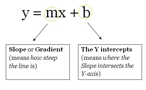
y = mx + b

Imagine having multiple of these. Since now, you will be computing multiple outputs for the same data-point(input). These outputs then get sent to another unit as well which then computes the final output of the NN.

If all of this flew past you then, keep reading and you should be able to understand more.

Weights / Parameters / Connections

Being the most important part of an NN, these(and the biases) are the numbers the NN has to learn in order to generalize to a problem. That is all you need to know at this point.

Biases

These numbers represent what the NN “thinks” it should add after multiplying the weights with the data. Of course, these are always wrong but the NN then learns the optimal biases as well.

Hyper-Parameters

These are the values which you have to manually set. If you think of an NN as a machine, the nobs that change the behavior of the machine would be the hyper-parameters of the NN.

You can read another one of my articles here(Genetic Algorithms + Neural Networks = Best of Both Worlds) to find out how to make your computer learn the “optimal” hyper-parameters for an NN.

Activation Functions

These are also known as mapping functions. They take some input on the x-axis and output a value in a restricted range(mostly). They are used to convert large outputs from the units into a smaller value — most of the times — and promote non-linearity in your NN. Your choice of an activation function can drastically improve or hinder the performance of your NN. You can choose different activation functions for different units if you like.

Here are some common activation functions:

Sigmoid:
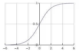
The Sigmoid function
Tanh:
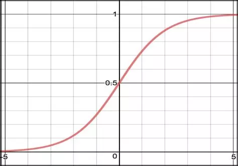
The tanh function
ReLU: Rectified Linear Unit:
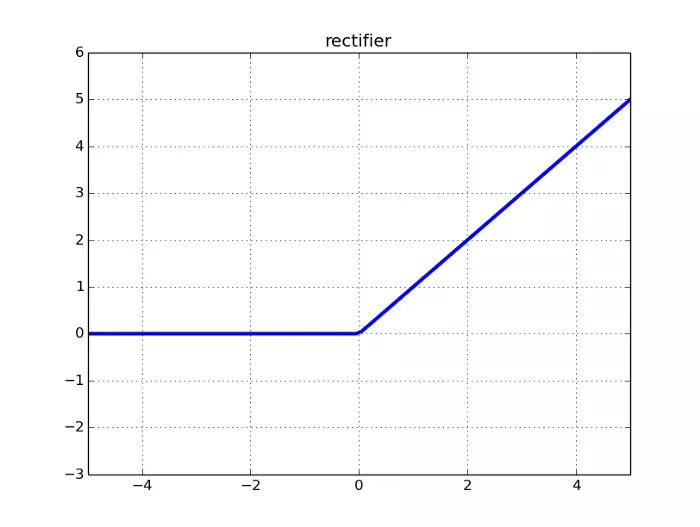
The ReLU function
Leaky ReLU:
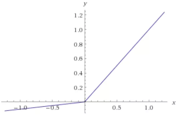
The Leaky ReLU function

Layers

These are what help an NN gain complexity in any problem. Increasing layers(with units) can increase the non-linearity of the output of an NN.

Each layer contains some amount of Units. The amount in most cases is entirely up to the creator. However, having too many layers for a simple task can unnecessarily increase its complexity and in most cases decrease its accuracy. The opposite also holds true.

There are 2 layers which every NN has. Those are the input and output layers. Any layer in between those is called a hidden layer. The NN in the picture shown below contains an input layer(with 8 units), an output layer(with 4 units) and 3 hidden layers with each containing 9 units.

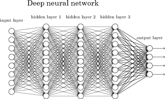
A Deep Neural Net

An NN with 2 or more hidden layers with each layer containing a large amount of units is called a Deep Neural Network which has spawned a new field of learning called Deep Learning. The NN shown in the picture is one such example.

What happens when a Neural Network Learns?

The most common way to teach an NN to generalize to a problem is to use Gradient Descent. Since I have already written an elaborate article on this topic which you can read to fully understand GD(Gradient Descent), I will not be explaining GD in this article. Here’s the GD article: Gradient Descent: All You Need to Know.

Coupled with GD another common way to teach an NN is to use Back-Propagation. Using this, the error at the output layer of the NN is propagated backwards using the chain rule from calculus. This for a beginner can be very challenging to understand without a good grasp on calculus so don’t get overwhelmed by it. Click here to view an article that really helped me when I was struggling with Back-Propagation. It took me over a day and a half to figure out what was going on when the errors were being propagated backwards.

There are many different caveats in training an NN. However, going over them in an article meant for beginners would be highly tedious and unnecessarily overwhelming for the beginners.

Implementation Details (How everything is manged in a project)

To explain how everything is managed in a project, I have created a JupyterNotebook containing a small NN which learns the XOR logic gate. Click here to view the notebook.

After viewing and understand what is happening in the notebook, you should have a general idea of how a basic NN is constructed.

The training data in the NN created in the notebook is arranged in a matrix. This is how data is generally arranged in. The dimensions of the matrices shown in different projects might vary.

Usually with large amounts of data, the data gets split into 2 categories: the training data(60%) and the test data(40%). The NN then trains on the training data and then tests its accuracy on the test data.

suryansh.xyz/