Gradient Descent is the most used learning algorithm in Machine Learning and this post will show you almost everything you need to know about it.
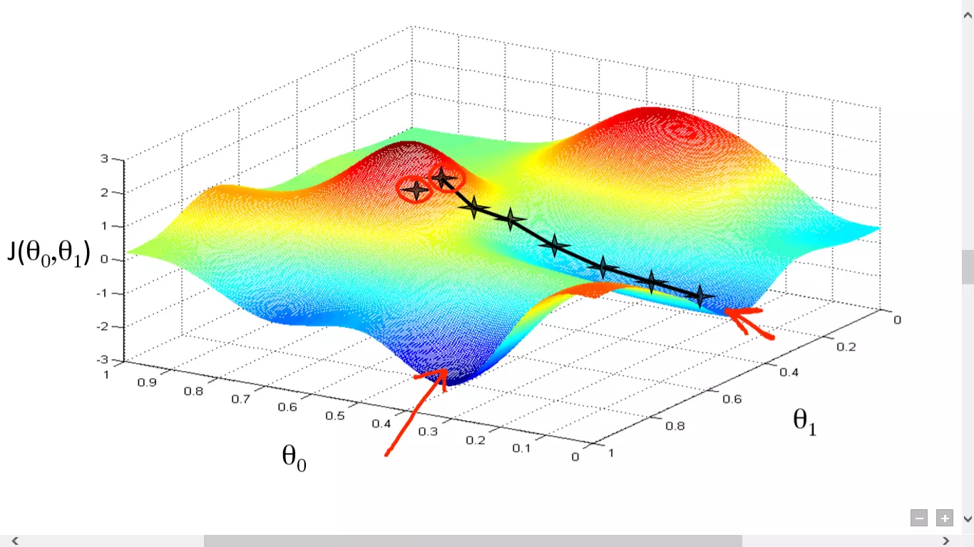
There are a few variations of the algorithm but this, essentially, is how any ML model learns. Without this, ML wouldn’t be where it is right now.
In this post, I will be explaining Gradient Descent with a little bit of math. Honestly, GD(Gradient Descent) doesn’t inherently involve a lot of math(I’ll explain this later). I’ll be replacing most of the complexity of the underlying math with analogies, some my own, and some from around the internet.
Here’s what I’ll be going over:
- The Point of GD: Explaining what the whole algorithm is.
- Different types of GD algorithms: Going over the different variations in GD.
- Code Implementation: Writing code in Python to demonstrate GD.
This is the first post of my “All You Need to Know” series on Machine Learning, in which, I do the research regarding an ML topic, for you. I then, condense everything I’ve learnt into a single post, for you to consume and hopefully learn from.
Lets get started!
1. The Point of GD
Gradient Descent requires a cost function(there are many types of cost functions). We need this cost function because we want to minimize it. Minimizing any function means finding the deepest valley in that function. Keep in mind that, the cost function is used to monitor the error in predictions of an ML model. So minimizing this, basically means getting to the lowest error value possible or increasing the accuracy of the model. In short, We increase the accuracy by iterating over a training data set while tweaking the parameters(the weights and biases) of our model.
So, the whole point of GD is to minimize the cost function.
The meat of the algorithm is the process of getting to the lowest error value. Analogically this can be seen as, walking down into a valley, trying to find gold(the lowest error value). While we’re at this, I’m sure you’ve wondered how we would find the deepest valley in a function with many valleys, if you can only see the valleys around you? I won’t be going over the ways to solve that problem as that is beyond of this post(meant for beginners). However, just know that there are ways to work around that problem.
Moving forward, to find the lowest error(deepest valley) in the cost function(with respect to one weight), we need to tweak the parameters of the model. How much do we tweak them though? Enter Calculus. Using calculus, we know that the slope of a function is the derivative of the function with respect to a value. This slope always points to the nearest valley!
Here(in the picture), we can see the graph of the cost function(named “Error” with symbol “J”) against just one weight. Now if we calculate the slope(let’s call this dJ/dw) of the cost function with respect to this one weight, we get the direction we need to move towards, in order to reach the local minima(nearest deepest valley). For now, let’s just imagine our model having just one weight.
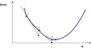
Cost Function “J” plotted against one weight.
When we iterate over all the training data, we keep adding dJ/dw for each weight. Since, the cost keeps changing depending on the training example, dJ/dw also keeps changing. We then divide the accumulated value by the no. of training examples to get the average. We then use that average(of each weight) to tweak each weight.
In essence, the cost function is just for monitoring the error with each training example while the derivative of the cost function with respect to one weight is where we need to shift that one weight in order to minimize the error for that training example. You can create models without even using the cost function. But you will have to use the derivative with respect to each weight (dJ/dw).
Now that we have found the direction we need to nudge the weight, we need to find how much to nudge the weight. Here, we use the Learning Rate. The Learning Rate is called a hyper-parameter. A hyper-parameter is a value required by your model which we really have very little idea about. These values can be learned mostly by trial and error. There is no, one-fits-all for hyper-parameters. This Learning Rate can be thought of as a, “step in the right direction,” where the direction comes from dJ/dw.
This was the cost function plotted against just one weight. In a real model, we do all the above, for all the weights, while iterating over all the training examples. In even a relatively small ML model, you will have more than just 1 or 2 weights. This makes things way harder to visualize, since now, your graph will be of dimensions which our brains can’t even imagine.
Going back to the point I made earlier when I said, “Honestly, GD(Gradient Descent) doesn’t inherently involve a lot of math(I’ll explain this later).” Well, it’s about time.
1.1. More on Gradients
With a cost function, GD also requires a gradient which is dJ/dw(the derivative of the cost function with respect to a single weight, done for all the weights). This dJ/dw depends on your choice of the cost function. There are many types of cost functions(as written above as well). The most common is the Mean-Squared Error cost function.

The derivative of this with respect to any weight is(this formula shows the gradient computation for linear regression):

This is all the math in GD. Looking at this, you can tell that inherently, GD doesn’t involve a lot of math. The only math it involves out of the box is multiplication and division which we will get to. This means, that your choice of a cost function, will affect your calculation of the gradient of each weight.
1.2. The Learning Rate.
Everything we talked about above, is all text book. You can open any book on GD and it will explain something similar to what I wrote above. Even the formulas for the gradients for each cost function can be found online without knowing how to derive them yourself.
The problem for most models however, arises with the learning rate. Let’s look at the update expression for each weight(j ranges from 0 to the amount of weight and Theta-j is the jth weight in a weight vector, k ranges from 0 to the amount biases where B-k is the kth bias in a bias vector). Here, alpha is the learning rate. From this, we can tell that, we’re computing dJ/dTheta-j(the gradient of weight Theta-j) and then we’re taking a step of size alpha in that direction. Hence, we’re moving down the gradient. To update the bias, replace Theta-j with B-k.
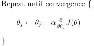
If this step size, alpha, is too large, we will overshoot the minimum, that is, we won’t even be able land at the minimum. If alpha is too small, we will take too many iterations to get to the minimum. So, alpha needs to be just right. This confuses many people and honestly, it confused me for a while as well.
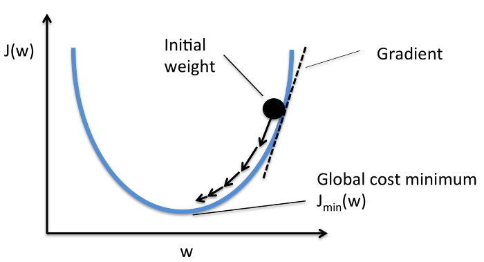
1.3. Summary
Well, that’s it. That’s all there is to GD. Let’s summarize everything in pseudo-code:
Note: The weights here are in vectors. In larger models they will probably be matrices. This example only has one bias but in larger models, these will probably be vectors.
-
for i = 0 to number of training examples:
- Calculate the gradient of the cost function for the i-th training example with respect to every weight and bias. Now you have a vector full of gradients for each weight and a variable containing the gradient of the bias.
- Add the gradients of the weights calculated to a separate accumulator vector which after you’re done iterating over each training example, should contain the sum of the gradients of each weight over the several iterations.
- Like the weights, add the gradient of the bias to an accumulator variable.
-
Now, AFTER iterating over all the training examples perform the following:
- Divide the accumulator variables of the weights and the bias by the number of training examples. This will give us the average gradients for all weights and the average gradient for the bias. We will call these the updated accumulators(UAs)
-
Then, using the formula shown below, update all weights and the bias. In place of dJ/dTheta-j you will use the UA(updated accumulator) for the weights and the UA for the bias. Doing the same for the bias.

This was just one GD iteration.
Repeat this process from start to finish for some number of iterations. Which means for 1 iteration of GD, you iterate over all the training examples, compute the gradients, then update the weights and biases. You then do this for some number of GD iterations.
2. Different Types of GDs
There are 3 variations of GD:
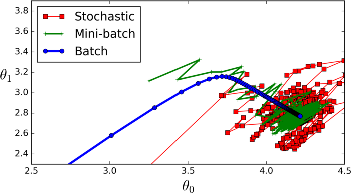
- Mini — Batch — GD: Here, instead of iterating over all training examples and with each iteration only performing computations on a single training example, we process n training examples at once. This is a good choice for very large data sets.
-
Stochastic — GD: In this, instead of using and looping over each training example, we use JUST USE ONE. There are a few things to note about this:
- With every GD iteration, you need to shuffle the training set and pick a random training example from that.
- Since, you’re only using one training example, your path to the local minima will be very noisey like a drunk man after having one too many drinks.
- Batch — GD: This is what we just discussed in the above sections. Looping over every training example, the vanilla(basic) GD.
Here’s a picture comparing the 3 getting to the local minima:
3. Code Implementation
In essence, using Batch GD, this is what your training block of code would look like(in Python).
    def train(X, y, W, B, alpha, max_iters):
        '''
        Performs GD on all training examples,
        X: Training data set,
        y: Labels for training data,
        W: Weights vector,
        B: Bias variable,
        alpha: The learning rate,
        max_iters: Maximum GD iterations.
        '''
        dW = 0 # Weights gradient accumulator
        dB = 0 # Bias gradient accumulator
        m = X.shape[0] # No. of training examples
        for i in range(max_iters):
            dW = 0 # Reseting the accumulators
            dB = 0
            for j in range(m):
                # 1. Iterate over all examples,
                # 2. Compute gradients of the weights and biases in w_grad and b_grad,
                # 3. Update dW by adding w_grad and dB by adding b_grad,
             W = W - alpha * (dW / m) # Update the weights
             B = B - alpha * (dB / m) # Update the bias

        return W, B # Return the updated weights and bias.
If this still seems a little confusing, here’s a little Neural Network I made which learns to predict the result of performing XOR on 2 inputs.